Try our free AI tools – no sign-up needed!


Frequency Distribution Table Calculator: Formula, Worked Example and Free Online Tool
Got a list of numbers? Paste it into the free frequency distribution table calculator online and get classes, frequencies, relative and cumulative percentages and a histogram in seconds, without login.
Jump to the free tool ↓A long list of raw numbers tells you very little. Thirty exam scores, two hundred delivery times or a thousand survey ages only start to make sense once you group them and count how many fall into each range. That grouped summary is a frequency distribution table, and a frequency distribution table calculator builds it for you without the tally marks, rounding mistakes or spreadsheet formulas.
This guide explains the frequency distribution formula step by step, works through a complete example by hand, shows how to read relative and cumulative frequency, and then walks you through the free Orixiva frequency distribution table calculator. It is a frequency distribution table calculator online without login, signin or signup, and it runs in your browser on a phone or computer.
Key takeaways
- A frequency table counts how many values fall into each class (range) of your data.
- Core formulas: class width = (max − lower limit) ÷ k; relative frequency = f ÷ n; cumulative frequency adds f down the table.
- If you are unsure how many classes to use, Sturges’ rule gives k = ⌈log₂ n + 1⌉: 6 classes for 30 values, 8 for 100.
- The modal class has the highest frequency; the median class is where the cumulative percentage passes 50%.
- The Orixiva calculator accepts up to 100,000 values, shows the working, draws a histogram and exports results, free and without login.
What is a frequency distribution table?
Quick answer: A frequency distribution table lists groups of values (classes) next to the number of observations in each group (the frequency). It turns raw data into a summary that shows where values cluster, how spread out they are and whether the shape is symmetric or skewed.
There are two common types:
Ungrouped frequency table
Each distinct value gets its own row.
x → f
- Shoe sizes, number of children, dice rolls
- Best for a few repeated values
Grouped frequency table
Values are grouped into equal-width classes.
40–50 → f
- Scores, heights, times, prices, ages
- Best for many different values
The Orixiva tool builds a grouped frequency table, because that is the version most people need for continuous data and the one that is slow to do by hand. For every class it reports the class range, midpoint, frequency (f), relative frequency, cumulative frequency and cumulative percentage, then highlights the modal class and draws a histogram.
The frequency distribution formula, step by step
There is no single “frequency distribution formula”. It is a short chain of formulas, each feeding the next. These are the exact rules the calculator uses.
1 · Number of classes (Sturges’ rule)
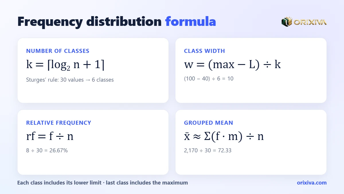
k = ⌈ log2 n + 1 ⌉
- n
- number of data values
- ⌈ ⌉
- round up to the next whole number
2 · Class width
w = (max − L) ÷ k
- max
- largest value in the data
- L
- lower limit of the first class (usually the minimum)
3 · Midpoint, relative and cumulative frequency
mi = (lower + upper) ÷ 2 · rfi = fi ÷ n · CFi = f1 + … + fi
- fi
- number of values in class i
- rfi
- share of all values, often shown as a percentage
- CFi
- running total from the first class to class i
4 · Grouped mean
x̄ ≈ Σ(fi × mi) ÷ n
- Σ
- sum over all classes
Two checks catch most errors: the frequencies must add up to n, and the last cumulative percentage must be 100%.
Worked example: a frequency table for 30 exam scores
A teacher has these 30 test scores out of 100:
42 47 51 55 58 59 61 63 64 66 67 68 69 70 72 73 74 75 76 78 79 81 82 84 85 88 90 93 96 100
- Count the values: n = 30.
- Choose the classes: Sturges gives k = ⌈log₂ 30 + 1⌉ = ⌈5.91⌉ = 6.
- Pick a tidy lower limit: the minimum is 42, so start at 40 to get round numbers.
- Class width: (100 − 40) ÷ 6 = 10, giving 40–50, 50–60 … 90–100.
- Count each class: each class includes its lower limit, so 70 goes in 70–80; the last class also includes the maximum, 100.
- Add the percentages: divide each f by 30 and keep a running total.
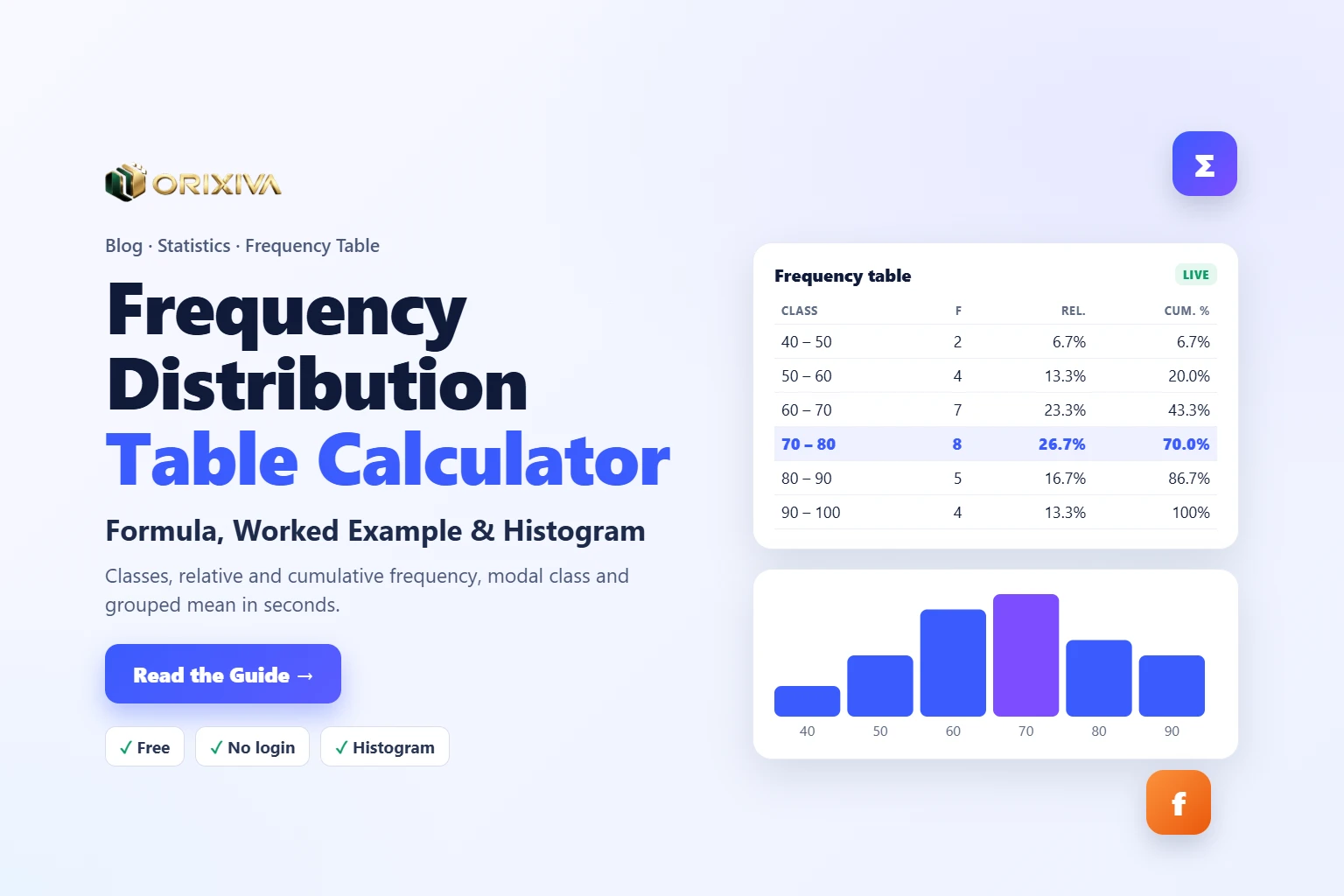
| Class | Midpoint | f | Relative | Cumulative | Cum. % |
|---|---|---|---|---|---|
| 40 – 50 | 45 | 2 | 6.67% | 2 | 6.67% |
| 50 – 60 | 55 | 4 | 13.33% | 6 | 20.00% |
| 60 – 70 | 65 | 7 | 23.33% | 13 | 43.33% |
| 70 – 80 (modal) | 75 | 8 | 26.67% | 21 | 70.00% |
| 80 – 90 | 85 | 5 | 16.67% | 26 | 86.67% |
| 90 – 100 | 95 | 4 | 13.33% | 30 | 100.00% |
| Total | 30 | 100% |
Plotting the frequencies as touching bars gives a histogram. The orange line joining the midpoints is a frequency polygon. The shape rises to a peak in 70–80 and falls off slightly more slowly to the right.
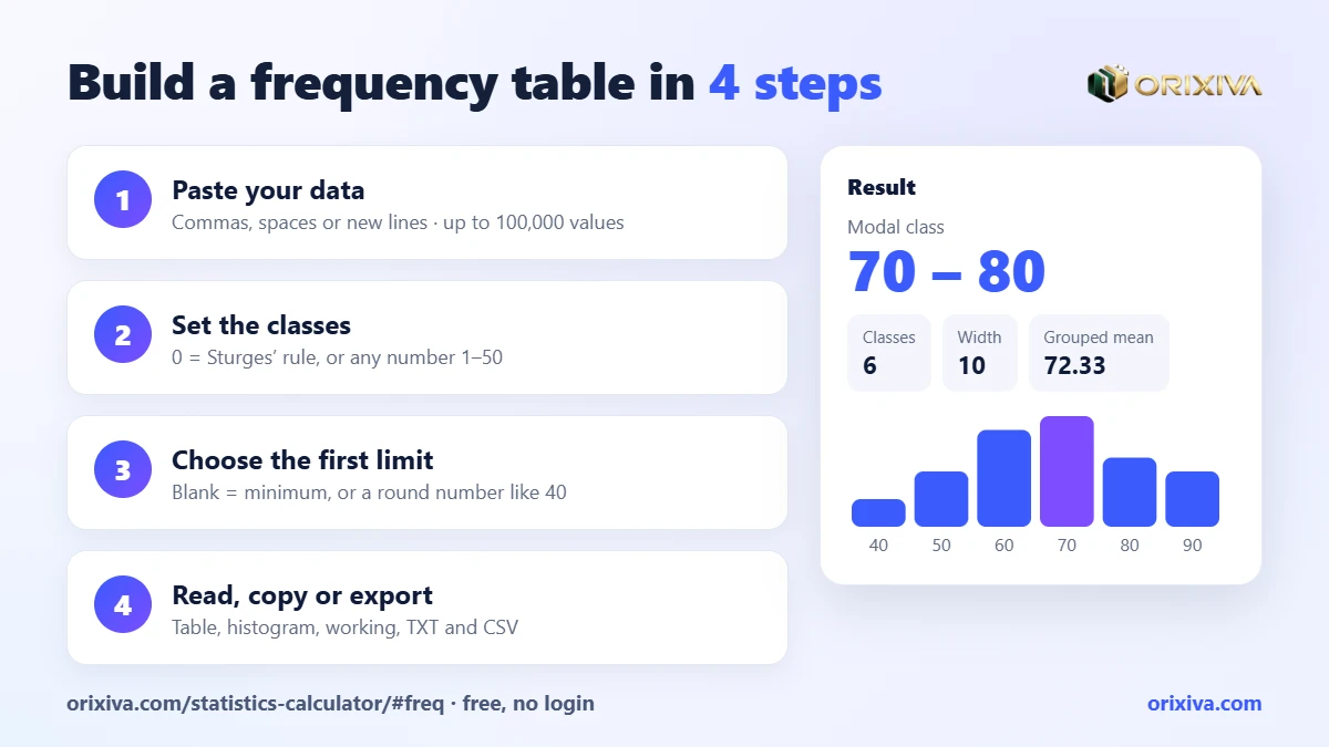
Classes6
Class width10
Modal class70 – 80
Grouped mean72.33
Check it in 20 secondsPaste the 30 scores into the frequency distribution table calculator, leave classes at 0 (Sturges) and type 40 as the first class lower limit. You should see exactly the table above, with the 70–80 row highlighted.
Flowchart: building any frequency table
- Collect the raw valuesOne number per observation; remove blanks and text
- Are there only a few distinct values?YesUse an ungrouped table: one row per valueNoGroup the values into classes
- Do you know how many classes you want?YesUse your k (5–15 is typical)NoUse Sturges: k = ⌈log₂ n + 1⌉
- Width = (max − lower limit) ÷ kRound the lower limit down for tidy class edges
- Tally f, then add relative and cumulative columnsf ÷ n, then running totals
- Check Σf = n and the last cumulative % = 100%Then draw the histogram and describe the shape
How many classes should a frequency table have?
Too few classes hide the shape; too many leave lots of classes with zero or one value. Sturges’ rule is a sensible default for small and medium data sets, and it is what the calculator uses when you leave the number of classes at 0.
Sturges’ rule: classes for different sample sizes
k = ⌈log₂ n + 1⌉. The number of classes grows slowly.
n = 10
5 classes
n = 20–31
6 classes
n = 50
7 classes
n = 100
8 classes
n = 500
10 classes
n = 1,000
11 classes
Bars to scale (11 classes = full width).
Other rules exist. The square-root rule uses k ≈ √n, and the Rice rule uses k ≈ 2·n1/3; both give more classes than Sturges for large data sets. In practice, try the default, then increase or decrease the number of classes until the histogram shows a clear, readable shape. The Orixiva calculator accepts any whole number from 1 to 50.
Large data setsFor thousands of values, Sturges can over-smooth a histogram. Try 15–30 classes and compare. If the bars become jagged and noisy, step back down.
Class limits, boundaries and where edge values go
The most common source of a wrong frequency table is a value sitting exactly on a class edge. Is a score of 70 in 60–70 or in 70–80? You need one consistent rule.
- Lower-inclusive rule (used by the calculator): each class includes its lower limit and excludes its upper limit, written [60, 70). A 70 goes into 70–80. The final class also includes the maximum, so nothing is left out.
- Textbook integer limits: some courses write 40–49, 50–59 for whole-number data. These are the same classes as [40, 50), [50, 60) for integers.
- Class boundaries: for 40–49, 50–59 the boundaries are 49.5 and 59.5. Histograms use boundaries so that the bars touch.
The tool lets you set the first class lower limit. Leave it blank to start at the minimum, or enter a round number (40 instead of 42) to get neater class edges. It must be less than or equal to the smallest value; otherwise the tool shows a clear error message.
How to read relative and cumulative frequency
The frequency column says “how many”. The other columns answer more useful questions:
Relative frequency
“What share of students scored 70–80?” 8 ÷ 30 = 26.67%. Relative frequencies let you compare groups of different sizes.
Cumulative frequency
“How many scored under 70?” Read the CF at the end of 60–70: 13 students.
Cumulative percentage
“What percentage scored under 80?” 70%. So 30% scored 80 or more.
Modal class
The class with the highest frequency, here 70–80. The calculator shows it as the headline result.
Plotting the cumulative percentage against the upper class boundary gives an ogive. Read across from 50% to find the median, or from 25% and 75% to estimate the quartiles.
Grouped mean and median from a frequency table
When you only have the frequency table (for example from a published report), you can still estimate the average and the median.
Grouped median
Median ≈ L + ((n/2 − CF) ÷ f) × w
- L
- lower limit of the median class
- CF
- cumulative frequency before the median class
- f, w
- frequency and width of the median class
For the exam scores, n/2 = 15, so the median class is 70–80 (the cumulative total passes 15 there). Median ≈ 70 + ((15 − 13) ÷ 8) × 10 = 72.5. The true median of the raw data is also 72.5.
The grouped mean is Σ(f × midpoint) ÷ n = (2×45 + 4×55 + 7×65 + 8×75 + 5×85 + 4×95) ÷ 30 = 2,170 ÷ 30 = 72.33. The true mean of the raw scores is 72.2. The small gap appears because grouping treats every value as if it sat at its class midpoint.
If you still have the raw data, use the Descriptive Statistics calculator in the same tool for the exact mean, median, standard deviation, quartiles and outliers.
How to use the free frequency distribution table calculator (step by step)
- Open the calculator. Go to the Orixiva frequency distribution table calculator. It opens with sample data loaded. No login, signin or signup is needed.
- Paste your data values. Separate numbers with commas, spaces, semicolons or new lines. You can paste a column straight from Excel or Google Sheets. At least 2 and up to 100,000 values are accepted.
- Set the number of classes. Leave 0 to use Sturges’ rule, or enter your own number from 1 to 50.
- Set the first class lower limit (optional). Leave it blank to start at the minimum, or enter a round number such as 0, 10 or 40.
- Read the results. They update as you type: modal class, number of classes, class width, number of values and grouped mean, then the full table with midpoint, f, relative, cumulative and cumulative % columns, and a histogram.
- Check the working. “How it was calculated” lists the class count rule, the width formula and how the relative and cumulative columns and the grouped mean were found.
- Save or share. Copy the result, download it as a TXT file or print it. Press Calculate to keep it in Recent calculations and export that list as CSV.
Everything runs in your browser. Your numbers are not uploaded to a server, which matters when the data are student marks, patient readings or customer records.
Who uses a frequency distribution table calculator?
Students
Check homework, build tables for projects and see the working for each column before an exam.
Teachers
Summarise class results, find the modal score band and show a histogram in a lesson.
Researchers
Describe survey ages, incomes or response times in the descriptive section of a thesis or report.
Quality teams
Group measurements such as weights or diameters to spot drift and values near specification limits.
Business analysts
Group order values, delivery times or ticket counts to see where most customers fall.
Health workers
Summarise ages, readings or waiting times privately, without uploading records.
Frequency tables in Excel and Google Sheets
Spreadsheets can build a frequency table, but you have to create the class edges yourself. With data in A2:A31 and upper class limits in C2:C7:
| Task | Formula |
|---|---|
| Count in a class [40, 50) | =COUNTIFS(A:A,">=40",A:A,"<50") |
| All frequencies at once (upper limits in C2:C7) | =FREQUENCY(A2:A31,C2:C7) |
| Relative frequency (f in D2) | =D2/SUM($D$2:$D$7) |
| Cumulative frequency | =SUM($D$2:D2) |
| Sturges’ classes | =ROUNDUP(LOG(COUNT(A2:A31),2)+1,0) |
Watch the edge ruleExcel’s FREQUENCY counts values less than or equal to each bin (upper-inclusive). The Orixiva calculator is lower-inclusive. Values sitting exactly on a class edge can therefore land in different classes. Neither is wrong; just state which rule you used.
Spreadsheet
Flexible, but manual.
5 formulas
- You build the bins
- Separate chart setup
Orixiva calculator
Paste and read.
1 paste
- Classes, width, %, histogram
- Working shown, CSV export
Mistakes to avoid with frequency tables
Overlapping classes
Classes such as 40–50 and 50–60 must follow one edge rule, or a 50 gets counted twice or not at all.
Unequal class widths
Unequal widths distort a histogram because wide classes collect more values. Keep widths equal unless you are plotting frequency density.
Forgetting the total check
If Σf is not n, a value is missing or double-counted. The calculator shows n so you can compare it with your source.
Reading the modal class as the mode
The modal class is a range, not a single value. With the raw data, the mode can sit outside the modal class.
Treating the grouped mean as exact
The grouped mean is an estimate. Report the raw-data mean when you have the raw values.
For deeper background on histograms, relative histograms and cumulative histograms, the NIST/SEMATECH e-Handbook of Statistical Methods has a clear reference page.
Your turn: What data are you grouping: scores, ages, times or sales? Tell us your sample size and how many classes looked best in the comments, so other readers can learn from your example.
Build your frequency table now
Paste your numbers, choose the classes and get the full frequency distribution table with relative and cumulative percentages, a histogram and the working. Free online without login, and nothing leaves your browser.
Open the frequency table calculator → Need a different statistics or math tool? Search on orixiva.comRelated guides: normal distribution calculator online, confidence interval calculator online, sample size calculator, t-test and p-value explained and how to calculate percentage.
Frequency distribution questions people often ask
Is there a frequency distribution table calculator online without login?
Yes. The Orixiva frequency distribution table calculator is free, needs no login, signin or signup, and runs in any modern browser.
What is the frequency distribution formula?
It is a set of steps: choose k classes (Sturges: ⌈log₂ n + 1⌉), width = (max − lower limit) ÷ k, count f in each class, relative frequency = f ÷ n, and cumulative frequency = running total of f.
How do I find the class width?
Subtract the first class lower limit from the maximum and divide by the number of classes. For scores from 40 to 100 in 6 classes, width = 60 ÷ 6 = 10.
What is the difference between frequency and relative frequency?
Frequency is a count (8 students). Relative frequency is that count as a share of the total (8 ÷ 30 = 26.67%).
How is cumulative frequency calculated?
Add each class frequency to the total of all the classes before it. The last cumulative frequency always equals n.
Which class does a value on the boundary go in?
In the Orixiva calculator, each class includes its lower limit, so 70 goes in 70–80. The last class also includes the maximum.
How many values can I paste?
From 2 up to 100,000 numbers, separated by commas, spaces, semicolons or new lines.
Does the calculator draw a histogram?
Yes. A histogram of the same classes appears under the frequency table, and the modal class row is highlighted.
Can I estimate the median from a frequency table?
Yes. Use Median ≈ L + ((n/2 − CF) ÷ f) × w for the class where the cumulative frequency first reaches n/2.
Is my data uploaded anywhere?
No. The calculations run in your browser, and your numbers are not sent to or stored on Orixiva’s server.
Can I export the frequency table?
You can copy the result, download it as a TXT file, print it, and export your saved calculations as CSV.
Does it work on a phone?
Yes. The calculator works in mobile browsers with no app to install.