Try our free AI tools – no sign-up needed!


Normal Distribution Calculator Online: How to Find Probabilities, Z-Scores and Percentiles
Need a probability now? The free normal distribution calculator online finds P(X < a), P(X > a), between, outside and inverse percentiles with a shaded bell curve, without login.
Jump to the free tool ↓Test scores, heights, machine fill weights and measurement errors often follow a familiar bell shape. Once you know the mean and standard deviation, the normal distribution tells you how likely any range of values is: what share of students score above 85, how many bottles are under-filled, or which height marks the top 10%.
This guide explains how to find normal distribution probabilities by hand with z-scores, shows five worked examples with charts, and walks you through the free Orixiva normal distribution calculator. It is a normal distribution calculator online without login, signin or signup: you type three numbers and read the answer, the shaded curve and the working.

Key takeaways
- A normal distribution is described by two numbers: the mean μ (centre) and the standard deviation σ (spread).
- Standardise first: z = (x − μ) ÷ σ. Then P(X < x) = Φ(z), the standard normal cumulative probability.
- Empirical rule: 68.27% of values lie within ±1σ, 95.45% within ±2σ and 99.73% within ±3σ.
- For percentiles, reverse it: x = μ + z·σ. The 95th percentile is μ + 1.645σ.
- The Orixiva calculator handles below, above, between, outside and inverse questions, free and without login.
What is a normal distribution?
Quick answer: A normal distribution is a symmetric, bell-shaped probability distribution. Most values sit near the mean, and values become steadily less likely the further they are from it. Its total area is 1 (100%), so the area under the curve over any range is the probability of that range.
Three properties make it easy to work with:
- Symmetry: the mean, median and mode are equal, and the curve is a mirror image on each side.
- Two parameters: knowing μ and σ is enough to answer any probability question.
- Standardisation: every normal distribution can be converted to the standard normal (μ = 0, σ = 1) with a z-score, so one table or one function covers them all.
The normal model also matters beyond raw data. Averages of large samples tend to be approximately normal even when individual values are not (the central limit theorem), which is why it appears in confidence intervals and many hypothesis tests.
Normal distribution formulas you need
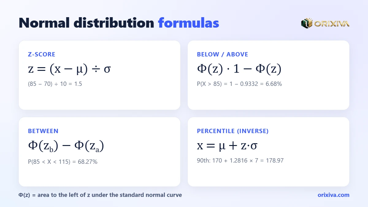
1 · Z-score (standardise)
z = (x − μ) ÷ σ
- x
- the value you are asking about
- μ
- mean of the distribution
- σ
- standard deviation (not the variance)
2 · Cumulative probability
P(X < x) = Φ(z) · P(X > x) = 1 − Φ(z)
- Φ(z)
- area under the standard normal curve to the left of z
3 · Between and outside two values
P(a < X < b) = Φ(zb) − Φ(za) · outside = 1 − between
- za, zb
- z-scores of the lower and upper values
4 · Inverse (percentile to value)
x = μ + z·σ, where z = Φ−1(p)
- p
- cumulative probability, e.g. 0.90 for the 90th percentile
Probability density function (the curve itself)
f(x) = e−(x − μ)²/(2σ²) ÷ (σ√(2π))
- f(x)
- height of the curve; probabilities are areas, not heights
Φ(z) has no simple closed form, which is why people used printed z-tables. The Orixiva calculator evaluates it numerically with a double-precision algorithm, so you get results to four decimal places of a percent.
The 68–95–99.7 rule (empirical rule)
Share of values within k standard deviations
Exact values for any normal distribution.
μ ± 1σ
68.27%
μ ± 2σ
95.45%
μ ± 3σ
99.73%
Outside ±3σ: about 0.27%, roughly 1 value in 370.
Use the rule for quick mental checks. If test scores have μ = 100 and σ = 15, about 68% of people score between 85 and 115 and about 95% between 70 and 130. A score of 145 is 3σ above the mean, so it is rare.
How to find normal distribution probability: 5 question types
Almost every normal distribution question is one of five types. The calculator has a mode for each:
| Question | Notation | Formula | Calculator mode |
|---|---|---|---|
| Below a value | P(X < a) | Φ(za) | P(X < a) |
| Above a value | P(X > a) | 1 − Φ(za) | P(X > a) |
| Between two values | P(a < X < b) | Φ(zb) − Φ(za) | P(a < X < b) |
| Outside two values | P(X < a or X > b) | Φ(za) + 1 − Φ(zb) | P(X < a or X > b) |
| Value for a percentile | x for P(X < x) = p | μ + Φ−1(p)·σ | x for a given cumulative probability |
For a continuous distribution, P(X < a) and P(X ≤ a) are the same, because the probability of hitting one exact value is zero.
Five worked normal distribution examples
Example 1: below a value
Scores have μ = 100 and σ = 15. What share score below 85?
- z = (85 − 100) ÷ 15 = −1.
- Φ(−1) = 0.1587.
- P(X < 85) = 15.87%, about 1 person in 6.3.
Example 2: above a value
Exam marks have μ = 70 and σ = 10. What share score above 85?
- z = (85 − 70) ÷ 10 = 1.5.
- Φ(1.5) = 0.9332, so 1 − 0.9332 = 0.0668.
- P(X > 85) = 6.68%. In a class of 150, expect about 10 students above 85.
Example 3: between two values
Using μ = 100 and σ = 15 again, what share score between 85 and 115?
- za = −1 and zb = 1.
- Φ(1) − Φ(−1) = 0.8413 − 0.1587 = 0.6827.
- P(85 < X < 115) = 68.27%, the first part of the empirical rule.
Example 4: outside two values (quality control)
A machine fills bottles with μ = 500 ml and σ = 4 ml. Bottles outside 492–508 ml are rejected. What is the reject rate?
- z = (492 − 500) ÷ 4 = −2 and z = (508 − 500) ÷ 4 = 2.
- Outside = Φ(−2) + 1 − Φ(2) = 0.0228 + 0.0228.
- P(outside) = 4.55%: about 455 rejects per 10,000 bottles.
Example 5: inverse, value for a percentile
Adult heights in a group have μ = 170 cm and σ = 7 cm. What height marks the 90th percentile?
- Φ−1(0.90) = 1.2816.
- x = 170 + 1.2816 × 7 = 178.97.
- The 90th percentile is about 179.0 cm. 10% of the group is taller.
Try it in the calculatorChoose “x for a given cumulative probability”, enter mean 170, standard deviation 7 and probability 90. The result is 178.97, with z = 1.28155, an upper tail of 0.1, and the symmetric 80% interval 161.03 to 178.97.
Below 85 (μ 100, σ 15)15.87%
Above 85 (μ 70, σ 10)6.68%
Outside 492–5084.55%
90th percentile height178.97 cm
Flowchart: which normal distribution question are you asking?
- Write down μ and σUse the standard deviation, not the variance
- Do you know a value and want a probability?YesForward question: go to the next stepNo, I know a %Inverse: x = μ + Φ⁻¹(p)·σ
- One value or two?OneBelow → Φ(z); above → 1 − Φ(z)TwoBetween → Φ(z_b) − Φ(z_a); outside → 1 − between
- Standardise each value: z = (x − μ) ÷ σThen look up Φ(z) or let the calculator do it
- Sense-check with the 68–95–99.7 ruleA z beyond ±3 should give a tiny probability
Z-table quick reference
These standard normal values come up again and again in statistics:
| z | Φ(z) = P(Z < z) | Upper tail | Common use |
|---|---|---|---|
| 0 | 0.5000 | 0.5000 | The mean is the median |
| 1 | 0.8413 | 0.1587 | One standard deviation |
| 1.282 | 0.9000 | 0.1000 | 90th percentile; 80% confidence |
| 1.645 | 0.9500 | 0.0500 | 95th percentile; 90% confidence |
| 1.960 | 0.9750 | 0.0250 | 95% confidence intervals |
| 2.326 | 0.9900 | 0.0100 | 99th percentile; 98% confidence |
| 2.576 | 0.9950 | 0.0050 | 99% confidence intervals |
| 3 | 0.9987 | 0.0013 | Three-sigma limits |
For negative z, use symmetry: Φ(−z) = 1 − Φ(z).
How to use the free normal distribution calculator (step by step)
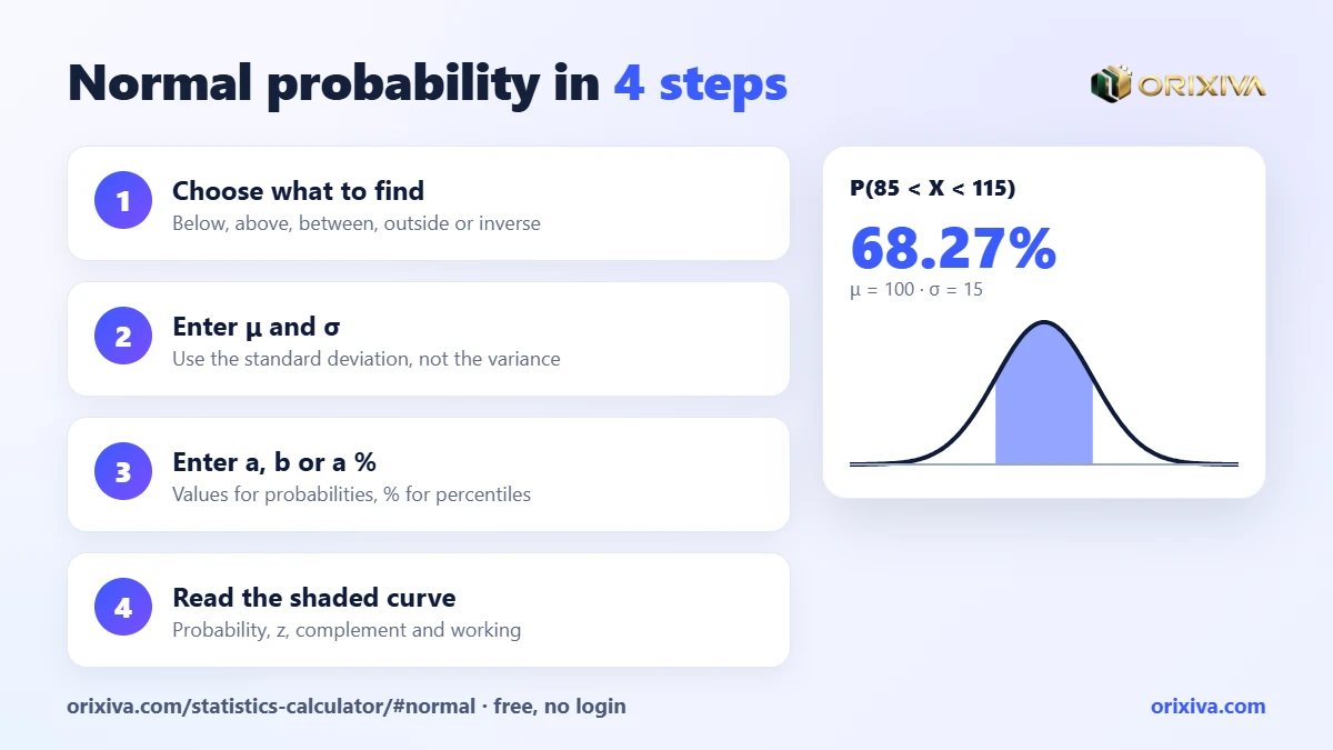
- Open the calculator. Go to the Orixiva normal distribution calculator. It opens with μ = 100, σ = 15 and a = 85. No login, signin or signup.
- Choose what to find. P(X < a), P(X > a), P(a < X < b), P(X < a or X > b), or x for a given cumulative probability. Only the fields you need are shown.
- Enter the mean and standard deviation. The standard deviation must be positive.
- Enter the value(s) or the percentile. For between and outside, b must be greater than a. For the inverse, type the cumulative probability as a percentage, such as 95.
- Read the result. The probability appears as a percentage, with the decimal probability, the z-score, the complement and a “1 in …” figure. The inverse mode shows x, z, the upper tail and the symmetric interval.
- Look at the shaded curve. A bell chart shades exactly the region you asked about, which is the fastest way to catch a wrong tail.
- Check, save or share. “How it was calculated” shows the standardising step. Copy the result, download a TXT file or print it; press Calculate to keep it in Recent calculations and export them as CSV.
Results update as you type, and everything runs in your browser on a phone, tablet or computer.
Who uses a normal distribution calculator?
Students
Check z-table homework, see the shaded area and learn the steps instead of only the answer.
Teachers
Show how changing μ or σ moves and stretches the curve, live in class.
Quality engineers
Estimate the share of parts outside tolerance from the process mean and standard deviation.
HR and education
Turn scores into percentiles and set cut-offs such as the top 10%.
Researchers
Find critical values and tail probabilities for z-based methods.
Operations teams
Estimate how often delivery or waiting times exceed a target, such as 40 minutes.
Is your data really normal?
The calculator assumes a normal model. Before relying on it, check that the assumption is reasonable:
- Look at the shape. Build a histogram with the frequency distribution table calculator. It should be roughly symmetric with one peak.
- Check skewness. The Descriptive Statistics calculator reports skewness and kurtosis. Values near 0 suggest a normal-like shape.
- Watch the limits. Times, prices and incomes cannot be negative and are often right-skewed; a normal model can then underestimate long upper tails.
- Use the exact model for counts. For counts of successes, use the binomial or Poisson calculators in the same tool.
The NIST/SEMATECH e-Handbook page on the normal distribution gives the formal definitions and notes why it is so widely used.
Normal vs t, binomial and Poisson distributions
The normal curve is not the right model for every question. Choosing the wrong distribution is a bigger error than any rounding, so use this table to pick the right calculator:
| Distribution | Data type | Use it when | Example |
|---|---|---|---|
| Normal | Continuous | Values are symmetric around a mean and σ is known or well estimated | Heights, fill weights, test scores |
| Student’s t | Continuous | You estimate σ from a small sample (roughly under 30) | Mean of 12 lab measurements |
| Binomial | Counts out of n | Fixed number of yes/no trials with the same success chance | Defective items in a batch of 50 |
| Poisson | Counts per interval | Events happen independently at an average rate | Calls per hour, typos per page |
The t distribution looks like a normal curve with heavier tails; as the sample grows it becomes almost identical to the normal. For large n, the binomial can also be approximated by a normal curve with μ = np and σ = √(np(1 − p)), but the exact binomial calculator avoids the approximation altogether.
Real-life check: delivery timesA courier’s delivery times average 30 minutes with σ = 6. The normal model says P(X > 40) = 4.78%, about 1 delivery in 21. If your records show far more late deliveries than that, the times are probably right-skewed, and the normal model is underestimating the long tail.
Normal distribution in Excel and Google Sheets
| Task | Formula | Example result |
|---|---|---|
| P(X < 85), μ 100, σ 15 | =NORM.DIST(85,100,15,TRUE) | 0.1587 |
| P(X > 85), μ 70, σ 10 | =1-NORM.DIST(85,70,10,TRUE) | 0.0668 |
| Between 85 and 115 | =NORM.DIST(115,100,15,TRUE)-NORM.DIST(85,100,15,TRUE) | 0.6827 |
| 90th percentile, μ 170, σ 7 | =NORM.INV(0.9,170,7) | 178.97 |
| Z-score | =STANDARDIZE(85,70,10) | 1.5 |
| Φ(z) | =NORM.S.DIST(1.96,TRUE) | 0.9750 |
Spreadsheets give the number but not the picture. The calculator adds the shaded curve, the z-score and the complement in one view.
Mistakes to avoid
Using the variance instead of the standard deviation
If a source says “variance 225”, σ is √225 = 15. Entering 225 makes the curve far too wide.
Picking the wrong tail
“At least 85” is an above question; “at most 85” is a below question. The shaded chart makes this visible.
Mixing percent and decimal
The inverse mode asks for a percentage (90), not 0.9. The result also shows the decimal probability so you can copy either form.
Applying the normal model to skewed data
Tail probabilities are only as good as the model. Check the shape first, especially for extreme percentiles.
Rounding z too early
Rounding z to one decimal can shift a tail probability noticeably. Keep full precision until the final answer.
Your turn: What are you modelling with a bell curve: exam scores, heights, fill weights or something else? Share your mean, standard deviation and question in the comments, and we will help other readers learn from it.
Find any normal probability now
Enter the mean, standard deviation and value to get below, above, between, outside or percentile answers with a shaded bell curve and the working. It is a normal distribution calculator online without login, and nothing leaves your browser.
Open the normal distribution calculator → Looking for a z-score, t-test or another calculator? Search on orixiva.comRelated guides: frequency distribution table calculator, confidence interval calculator online, sample size calculator and t-test and p-value explained. For z-scores of single values, use the z-score and percentile calculator.
Normal distribution questions people often ask
Is there a normal distribution calculator online without login?
Yes. The Orixiva normal distribution calculator online without login is free, needs no login, signin or signup, and works in any modern browser.
How do I find a normal distribution probability?
Convert the value to a z-score with z = (x − μ) ÷ σ, then find Φ(z) for “below”, 1 − Φ(z) for “above”, or subtract two Φ values for “between”.
What does the calculator need?
The mean, the standard deviation and either one or two values, or a cumulative percentage for the inverse mode.
How do I find the value for a percentile?
Use x = μ + z·σ with z = Φ⁻¹(p). In the calculator, choose “x for a given cumulative probability” and type the percentile.
What is the 68–95–99.7 rule?
For a normal distribution, 68.27% of values lie within one standard deviation of the mean, 95.45% within two and 99.73% within three.
What is the difference between normal and standard normal?
The standard normal has mean 0 and standard deviation 1. Any normal distribution becomes standard normal after converting values to z-scores.
Is P(X < a) the same as P(X ≤ a)?
Yes, for a continuous distribution such as the normal. The probability of one exact value is zero.
Can the probability be more than 100%?
No. Probabilities run from 0 to 1 (0% to 100%). If you get more, check the formula or the inputs.
How accurate is the calculator?
It evaluates the normal CDF numerically in double precision and shows probabilities to four decimal places of a percent, which is more precise than a printed z-table.
Does it work on a phone?
Yes. It runs in mobile browsers with no app, and your inputs are not sent to Orixiva’s server.
Can I save my results?
Yes. Copy the result, download it as a TXT file, print it, or save calculations to Recent calculations and export them as CSV.



[…] guides: normal distribution calculator online, confidence interval calculator online, sample size calculator, t-test and p-value explained and […]